Allen Bradley and siemens IP configuration and IoT module settings

AB:
1. USE usb2RS232 cable to connect to the CPU. CPU is connected to Ethernet module, ControlNet module and device Net module.

2. Open RSlinx. Delete all previous drivers(if cannot delete just restart Rslinx while everything is disconnected)!!! Configure a driver called RS-232 DF1 drivers. Select correct COM and baud rate to establish the driver. Should be able to see all the above devices in RSwho under this driver. Then select the Ethernet module, right click to change the properties, where we can set the IP and subnet mask for the Ethernet module.

3. Still in RSlinx, configure a driver for Ethernet. The name of driver is "Ethernet devices". When configure it there will be a window pop out asking for the IP address, put the address you set in step 2 into station 0, click okay. Then all above devices on the same backplane will have the same IP address will show up in RSWho.

3. Open RSLOGIX5000, should be able to see the devices on the same chassis in WhoActive.


SIEMENS:
1. ALL IP SETTINGS CAN BE DONE IN TIA PORTAL as long as the PLC is connected with Ethernet to the computer(workstation).
2.open TIA portal, first create the project without a in-predefined device, then start device detection
3.after successfully detected of the device, go to the project tree and select "online & diagnostics", in the menu we have a lot of options such as assign IP address or formatting the SD card, etc...


For using the IoT module for siemens PLC:
1. for setting the IP address and subnet mask: please refer to IoT2000 setup in the google drive(miles.luo.xl@google.com). The firmware of IoT2000 is dumped to the SD card and then used in the IoT2040 module in my case. It works.....

2. For installing the node-red please refer to the PDF showing the steps(miles.luo.xl@google.com). One thing to note is that all installations should be with the internet connection of the IoT module! Installing the nodes for S7 communication and Azure IoT-hub then. Refer to the PDF or go to the website of node-red. If it somehow doesn't work just simply format the SD card in TIA portal!

The code to start node red in the IoT module's OS: node /usr/lib/node_modules/node-red/red &
Current flow is stored at /home/root/.node-red/ can ls and rm the undesired flow (the folder is invisible for WINscp)

3. Follow the setting in this video to set up a flow. S7 reading value------>construct a payload string in correct format------>upload to IoT using the Azure IoT hub node. Done! The thing is to correctly construct a payload string in the correct format.

{
  "deviceId": "testenode1",
  "key": "cw3nniq77BbjpOCDLqb7xEFTU509HeR6Ki1NwR20jj0=",
  "protocol": "amqp",
  "data": "{tem: 25, wind: 20}"
}

4. Use the flow in this link to register the device in IoT hub:https://flows.nodered.org/node/node-red-contrib-azure-iot-hub. After registering we will have a key to access the hub.

For using the IoT module with AB PLC:

坐标变换学习

行星系坐标变换 和 一些 OPENGL的感悟

这个例子是地球绕太阳，月亮同时绕地球的渲染

1.太阳为原点渲染，地球的坐标先平移，再绕原点y轴旋转渲染
2.麻烦的是月亮。月亮的坐标上传后也以原点为中心（big bang模式！opengl的模型上传之后，其局部坐标和世界坐标是重合的，后续的变换都是在世界坐标系中进行的！就像宇宙形成一样从中心大爆炸！）


    1）月亮变换第一种方法：先缩放，然后偏移（偏移距离是月亮距离原点（即太阳）的绝对距离），然后进行坐标系变换，将此时的坐标（在太阳坐标系中给出）变换到地球坐标系中去。由于地球的坐标系是在太阳坐标系的基础上，先旋转再平移得到的（注意两者都有！），所以构建两个view变换矩阵，一个是旋转，一个是平移，月亮的太阳坐标先乘以旋转再乘以平移，得到月亮在地球坐标系里的坐标。（最后为了render，还要将这个坐标变换回太阳坐标系去，同样乘以两个view矩阵，不过和第一步的是相反的方向）。总体是一个世界到local，做完旋转在回到世界的变换过程。

    2） 第二种方法，月亮的坐标先缩放，再偏移，不过此时的偏移量按照相对地球的距离进行。然后做旋转，此时月亮是围绕中心轴以相对地球的偏移在旋转（这些变换都是在太阳坐标系下进行的）。接下来将旋转之后的坐标变换到地球坐标系中去，同样需要一个旋转一个平移变换，得到月亮在地球坐标系的坐标。最后再用两个相反的矩阵将这个坐标变换会太阳坐标系用于render。整体上是一个先在世界坐标系做完旋转（注意此时的旋转半径是月亮相对地球的距离），变换到local坐标，然后再回到世界的过程。

上述变换和在hexapod设计中的坐标变换是类似的（将旋转平台的坐标变换到base坐标系中去，而base坐标系是由旋转坐标系先旋转再平移得到的，所以构建两个view变换矩阵来做变换）

要记住view变换（坐标系变换）和坐标变换之间的关系！

opengl glutPostRedisplay(void)

1用法编辑

void glutPostRedisplay(void);

2描述编辑

glutPostRedisplay 标记当前窗口需要重新绘制。通过glutMainLoop下一次循环时，窗口显示将被回调以重新显示窗口的正常面板。多次调用glutPostRedisplay，在下一个显示回调只产生单一的重新显示回调。

为了便于理解，用下面的例子^[1]来说明：

假设有绘制代码：

glutDisplayFunc(display); // opengl drawing goes here

glutTimerFunc(30, drive, -1);// physics, movement equations here

glutMainLoop();

另外有代码如下：

void drive (int data)

{

glutTimerFunc(30, drive, -1);// call drive() again in 30 milliseconds

glutPostRedisplay();

}

如果有glutpostredisplay，mianloop运行的过程会像下面这样：

drive (-1);

display();

drive (-1);

display();

drive (-1);

display();

...

如果没有glutPostRedisplay，glutMainloop运行的过程会像下面这样：

drive (-1);

drive (-1);

drive (-1);

...

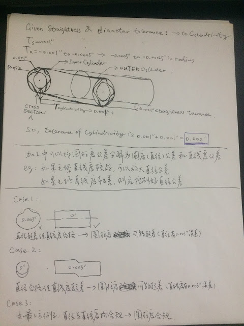
圆柱度 直线度 和直径公差关系推演

上述例子基于mcmaster的直线圆柱界面导轨数据： 直线度0.001"， 直径公差-0.001". 可见该导轨的圆柱度公差还是有可能达到0.002"。

数据结构与算法--fibonacci的动态规划解法

对比下面这个用一个数组来存储中间变量的方法：以下代码为JAVA：

1.    /** 
2.      * 自底向上包含"动态规划"思想的解法 
3.      * @param n 
4.      * @return 第n个斐波那契数 
5.      */  
6.     public static int downToTopReslove(int n) {  
7.         if(n == 0) {  
8.             return 0;  
9.         } else if(n == 1 || n == 2) {  
10.             return 1;  
11.         } else {  
12.             int[] fibonacciArray = new int[n+1]; //fibonacciArray[i]表示第i个斐波那契数  
13.             fibonacciArray[0] = 0;  
14.             fibonacciArray[1] = 1;  
15.             fibonacciArray[2] = 1;  
16.             for(int i=3;i<=n;i++) { //注意由于fibonacciArray[0]表示第0个元素，这里是i<=n，而不是i<n  
17.                 fibonacciArray[i] = fibonacciArray[i-1] + fibonacciArray[i-2];  
18.             }  
19.               
20.             return fibonacciArray[fibonacciArray.length-1];  
21.         }  
22.     }  

第一个算法只用了两个中间变量来存储中间值，每次值都会有变化，而第二个方法则是每个中间值都被存储在了对应的数组元素里。

上述两种算法都体现了动态规划的思想。

halfedge data structure

http://www.holmes3d.net/graphics/dcel/


C++ emplace_back:
https://www.kancloud.cn/wangshubo1989/vector/101113

emplace_back 可以在一个vector中添加一个新的object，这一添加可以免去调用该object的构造函数直接进行。

Cmake to find protobuf on windows

 I also struggled with this. To be more clear.

On Windows (7, similar on older windows): Start --> Control Panel --> System --> Advanced System Settings --> Environment Variables

Then either on the top panel or the bottom panel (if you want it to apply to other users do it on the bottom), create two new variables. The 1st one is

• CMAKE_INCLUDE_PATH which points at the bottom of your include path (should contain a "google" folder)
• CMAKE_LIBRARY_PATH which should contain "libprotobuf" "libprotobuf-lite" "liteprotoc" .lib files.

After you create the variables press OK and then re-start cmake (or clean the cache).

每个进程都会有一个返回值的. 
进程开始时是由系统的一个启动函数掉用了main函数的:   
int   nMainRetVal   =   main(); 
当从main函数退出后,启动函数便调用exit函数,并且把nMainRetVa传递给它. 
所以,任何时候都会调用exit函数的,正常情况下,main函数不会调用exit函数的,而是由return   0; 
返回值给nMainRetVal的,exit再接收这个值作为参数的.所以,正常情况下是以exit(0)退出的. 
如果,你程序发生异常,你可以在main函数中调用exit(1),强制退出程序,强制终止进程.其中1表示不正常退出

neural network

back propagation
http://www.cnblogs.com/charlotte77/p/5629865.html

matlab Neural network
http://blog.csdn.net/gongxq0124/article/details/7681000/

色度图 Chromacity Diagram

色度图：chromaticity diagram
http://netclass.csu.edu.cn/NCourse/hep089/Chapter4/CG_Txt_4_009.htm

色度图的马蹄形轮廓是如上所示的三刺激图在x,y,z三维空间中，可见光谱（380-700nm) 在x+y+z=1的平面上的的投影：

三刺激值可以理解为三个人为定义的原色对于某一可见光波长的拟合值，这一个值是一个百分比，代表各颜色所占的比例，用小写的x,y,z表示。有时候，这个值也可以被表示成各原色的值（相对值）。这时这三个值用X,Y,Z表示。

x,y,z与X,Y,Z的关系为：

图像的复原(Restoration）

图像退化的数学模型：

图像的退化是原图像经过一个退化系统之后的输出加上噪音：

g(x,y) = H[f(x,y)]+n(x,y)

其中H是退化函数，n是噪音。

对于H退化函数：

如果H系统是LTI（线性时不变系统，在图像领域成为线性空间不变），则可以用该系统的冲激响应来表征这一系统：

任意输入经过该系统H的输出可以表示为输入信号与H的单位冲激响应的卷积。

（再次说明卷积是求LTI输出的计算方法）。

反之，如果知道一张图经过退化后的输出，可以人为的用一个单位冲激作为输入，从而反解出H(u，v)。该计算在频域更为方便，因为卷积将变为乘法。

ALIASING

aliasing

一个信号，经过时间间隔T的采样， 然后傅里叶变换， 得到的结果是一个周期为1/T的函数。

如果2*1/T大于umax-umin，则不会产生混叠。

反之则不可能复原出原信号，混叠产生。

对于有限采样的（有限时间）信号，混叠是不可避免的，因为该类信号经过傅里叶变换之后是在频域无限拓展的（非带限的）。所以1/T*2不可能完全cover Umin和Umax的区间，混叠不可避免。处理的方法就是尽量在采样之前削弱信号的高频分量，如平滑图像，来减少高频区域的比重。

imshow matlab

1. matlab 中的double类型需要在0到1之间才能用imshow画出图来！uint8类型的数在0-255间可以用imshow;

fourier wraparound error

DFT是将一个有限的采样序列（无论是否周期）变化成为一个无线延拓的，周期的频率序列。

用盒状函数举例：

在频域：一个盒状函数（size n）

进行IDFT之后得到周期为N的无限延展的sinc函数。

同理，

一个频域一维图像（size=n)，IDFT之后也是一个周期为N的无限延展的函数。

频域滤波等同于盒状函数和该一维图像的相乘
由卷积定理，该滤波也等同于在时域的两个周期函数的卷积
这一卷积结果也是周期的（周期也为N）
所以，当周期N小于完整卷积所需的最小尺寸P时，所得的结果是存在error的，这一error就称为wraparound error.

解决这一问题的方法是对两个时域的周期为N的函数进行周期的延拓（零填充），使得size = P，其中P = 2N-1。通常会取偶数，即P = 2N。

简单说：
频域的filter和图像都是有限size的
经过IDFT之后变为无限延陀且周期的
这样两个无限的且周期的信号作卷积时，如果周期不够长，则卷积不完全
形成缠绕错误



实际处理中：
对图像延拓至size =P （二维下P*Q），然后直接构造一个等尺寸的频域滤波器，两者直接相乘。